Neural Networks in 100 lines of pure Python
Can we build a Deep learning framework in plain Python and Numpy? Can we make it compact, clear and extendable? Let's set out to explore those ideas and see what we can create!


Can we build a Deep learning framework in pure Python and Numpy? Can we make it compact, clear and extendable? Let's set out to explore those ideas and see what we can create!
In today's day and age, there are multiple frameworks to choose from, with various important features such as auto-differentiation, graph-based optimized computation, and hardware acceleration. It's easy to take those features for granted, but every once in a while peeking under the hood can teach us what makes things work and what doesn't.
What we'll cover:
- Automatic back-propagation
- How to implement a few basic layers
- How to create a training loop
If you want to jump straight to the code, feel free to scroll to the second half of the post or try it live in this Colab Notebook.
The design choices are heavily based on Thinc's Deep Learning library since they came up with the smart idea of using closures and the stack to share and keep track of intermediate results while calculating gradients. This post is also inspired by Jeremy Howard's great PyTorch tutorial, but taking it one more step towards the bottom getting rid of autograd.
A word on notation
Notation can often be a source of confusion, but it can also help us develop the right intuition. In the context of calculus for back propagation, we can focus on functions or on variables to think about derivatives. These are the edges and nodes in the computational graph. We will get to the same results either way, but I find that focusing on variables helps to make things more natural.
- Let $f:\mathbb{R}^n\to\mathbb{R}$ and $x\in\mathbb{R}^n$, then the gradient is the $n$-dimensional row vector of partial derivatives $\frac{\partial f}{\partial_j }(x)$
- If $f:\mathbb{R}^n\to\mathbb{R}^m$ and $x\in\mathbb{R}^n$ then the Jacobian matrix is an $m\times n$ matrix such that the $i^{\text{th}}$ is the gradient of $f$ restricted to the $i$ coordinate:
$$Jf(x)_{ij} = \frac{\partial f_i}{\partial_j}(x)$$ - For a function $f$ and two vectors $a$ and $b$ such that $a = f(b)$, whenever $f$ is clear from context we can write $\frac{\partial a}{\partial b}$ to denote the Jacobian $Jf$, or gradient if $a$ is a real number.
The chain rule
If we have three vectors in three vector spaces $a\in A$, $b\in B$, and $c\in C$ and two differentiable functions $f:A\to B$ and $g:B\to C$ such that $f(a) = b$ and $g(b) = c$ we can get the Jacobian of the composition as a matrix product of the Jacobian of $f$ and $g$:
$$\frac{\partial c}{\partial a} = \frac{\partial c}{\partial b} \cdot \frac{\partial b}{\partial a}$$
That's the chain rule in all its glory. The back-propagation algorithm, originally described in the '60s and '70s is the application of the chain rule to calculate gradients of a real function with respect to its various parameters.
Keep in mind that our end goal is to find a minimum (hopefully global) of a function by taking steps in the opposite direction of the said gradient, because locally at least this will take it downwards. This is how it looks when we have two parameters to optimize.
Reverse mode differentiation
If we compose many functions $f_i(a_i) = a_{i+1}$ instead of just two, then we can apply that formula repeatedly and conclude that
$$\frac{\partial a_n}{\partial a_1} = \frac{\partial a_n}{\partial a_{n-1}} \cdots \frac{\partial a_3}{\partial a_2}\cdot\frac{\partial a_2}{\partial a_1}$$
Of the many ways we can compute this product, the most common are from left to right or from right to left.
In practice, if $a_n$ is a scalar we will calculate the full gradient by starting with the row vector $\frac{\partial a_n}{\partial a_{n-1}}$ and multiplying by the Jacobians $\frac{\partial a_i}{\partial a_{i-1}}$ on the right one at a time. This operation is sometimes referred as VJP, or Vector-Jacobian Product. The whole process is known as reverse mode differentiation, because as intermediate results we gradually compute the gradients working from the last one $\frac{\partial a_n}{\partial a_{n-1}}$ backward through $\frac{\partial a_n}{\partial a_{n-2}}$, $\frac{\partial a_n}{\partial a_{n-3}}$, etc. In the end, we know the gradient of $a_n$ with respect to all other variables.
$$\frac{\partial a_n}{\partial a_{n-1}} \rightarrow \frac{\partial a_n}{\partial a_{n-2}} \rightarrow \cdots \rightarrow \frac{\partial a_n}{\partial a_1}$$
In contrast, forward mode does the exact opposite. It starts from one Jacobian like $\frac{\partial a_2}{\partial a_1}$ and multiplies on the left by $\frac{\partial a_3}{\partial a_2}$ to calculate $\frac{\partial a_3}{\partial a_1}$. If we keep multiplying by $\frac{\partial a_i}{\partial a_{i-1}}$ we'll gradually get the derivatives of all other variables with respect to $a_1$. When $a_1$ is a scalar, all the matrixes on the right side of the products are column vectors, and this is called a Jacobian-Vector Product (or JVP).
$$\frac{\partial a_n}{\partial a_1} \leftarrow\cdots\leftarrow \frac{\partial a_2}{\partial a_1} \leftarrow \frac{\partial a_2}{\partial a_1}$$
For back propagation, as you might have guessed, we are interested in the first of this two, since there's a single value we want on top, the loss function, derived with respect to multiple variables, the weights. Forward mode could still be used to compute those gradients, but it would be far less efficient since we would have to repeat the process multiple times.
This sounds like a lot of high-dimensional matrix products, but the trick is that very often the Jacobian matrixes will be sparse, block or even diagonal and, because we only care about the result of multiplying it by a row vector on the left, we won't need to compute or store it explicitly
In this article, we are focusing on a sequential composition of layers, but the same ideas apply to any algorithm or computational graph that we use to get to the result. Yet another nice description of reverse and forward mode in a more general context is given here.
Link to deep neural networks
In the typical setting for supervised machine learning, we have a big complex function that takes in a tensor of numerical features for our labeled samples, and several tensors that correspond to weights that characterize the model.
The loss, as a scalar function of both the samples and weights, is a measure of how far the model output was from the expected labels. We want to minimize it to find the most suitable weights. In deep learning, this function is expressed as a composition of simpler functions, each of which is easy to differentiate. All of them but the last are what we refer to as layers, and each layer usually has two sets of parameters: the inputs (which can be the output of the previous layer) and the weights.
The last function is the loss metric, which also has two sets of parameters: model output $y$ and the true labels $\hat{y}$. For example, if the loss metric $l$ is the mean square error then $\frac{\partial l}{\partial y}$ is $2\ \text{avg}(y - \hat{y})$. The gradient of the loss will be the starting row vector to apply reverse mode differentiation.
Autograd
The ideas behind Automatic Differentiation are quite mature. It can be done in runtime or during compilation, which can have a dramatic impact on performance. I recommend the HIPS autograd Python package for a thorough explanation of some of the concepts.
The core idea, however, is always the same, and we have known it ever since we started computing derivatives in school. If we can keep track of the computations that resulted in the final scalar output and we know how to differentiate each simple operation (sums and products, powers, exponentials, and logarithms, ...), we can recover the gradient of the output.
Let's say that we have some intermediate linear layer $f$ which is characterized by a matrix multiplication (let's leave the bias out for a sec):
$$y = f(x, w) = x\cdot w$$
In order to tune the values of $w$ with gradient descent, we need to compute the gradient $\frac{\partial l}{\partial w}$. The key observation that it's enough to know how changes in $y$ will affect $l$ to do that.
The contract that any layer has to satisfy is the following: if I tell you the gradient of the loss with respect to your outputs, you can tell me the gradient with respect to your inputs, which are in turn the previous layer outputs.
Now we can apply the chain rule twice: for the gradient with respect to $w$ we get that
$$\frac{\partial l}{\partial w} =\frac{\partial l}{\partial y}\cdot \frac{\partial y}{\partial w} = \frac{\partial l}{\partial y} \cdot x^t $$
and with respect to $x$
$$\frac{\partial l}{\partial x} =\frac{\partial l}{\partial y}\cdot \frac{\partial y}{\partial x} = \frac{\partial l}{\partial y} \cdot w $$
So we can both pass a gradient backward to enable previous layers to update themselves and update the internal layer weights to optimize the loss, and that's it!
Implementation time
Let's look at the code, or try it live in this Colab Notebook. We can start with a class that encapsulates a tensor and its gradients
class Parameter():
  def __init__(self, tensor):
    self.tensor = tensor
    self.gradient = np.zeros_like(self.tensor)
Now we can create the layer class, the key idea is that during a forward pass we return both the layer output and function that can receive the gradient of the loss with respect to the outputs and can return the gradient with respect to the inputs, updating the weight gradients in the process.
This is because while evaluating the model layer by layer there's no way to calculate the gradients if we don't know the final loss yet, instead the best thing you can do is return a function that CAN calculate the gradient later. And that function will only be called after we completed the forward evaluation, when you know the loss and you have all the necessary info to compute the gradients in that layer.
The training process will then have three steps, calculate the forward step, then the backward steps accumulate the gradients, and finally updating the weights. It’s important to do this at the end since weights can be reused in multiple layers and we don’t want to mutate the weights before time.
class Layer:
  def __init__(self):
    self.parameters = []

  def forward(self, X):
    """
    Override me! A simple no-op layer, it passes forward the inputs
    """
    return X, lambda D: D

  def build_param(self, tensor):
    """
    Creates a parameter from a tensor, and saves a reference for the update step
    """
    param = Parameter(tensor)
    self.parameters.append(param)
    return param

  def update(self, optimizer):
    for param in self.parameters: optimizer.update(param)
It's standard to delegate the job of updating the parameters to an optimizer, which receives an instance of a parameter after every batch. The simplest and most known optimization method out there is the mini-batch stochastic gradient descent
class SGDOptimizer():
  def __init__(self, lr=0.1):
    self.lr = lr

  def update(self, param):
    param.tensor -= self.lr * param.gradient
    param.gradient.fill(0)
Under this framework, and using the results we computed earlier, the linear layer looks like this snippet of code. We are using numpy overloaded @ operator for matrix multiplication.
class Linear(Layer):
  def __init__(self, inputs, outputs):
    super().__init__()
    tensor = np.random.randn(inputs, outputs) * np.sqrt(1 / inputs)
    self.weights = self.build_param(tensor)
    self.bias = self.build_param(np.zeros(outputs))

  def forward(self, X):
    def backward(D):
      self.weights.gradient += X.T @ D
      self.bias.gradient += D.sum(axis=0)
      return D @ self.weights.tensor.T
    return X @ self.weights.tensor +  self.bias.tensor, backward
Now, the next most used types of layers are activations, which are non-linear point-wise functions. The Jacobian of a point-wise function is diagonal, which means that when multiplied by the gradient it also acts a point-wise multiplication.
class ReLu(Layer):
  def forward(self, X):
    mask = X > 0
    return X * mask, lambda D: D * mask
A little harder is to compute the derivative of a Sigmoid, which is again applied pointwise:
class Sigmoid(Layer):
  def forward(self, X):
    S = 1 / (1 + np.exp(-X))
    def backward(D):
      return D * S * (1 - S)
    return S, backward
When we have many layers in a sequence, as we traverse them and get the successive outputs we can save the backward functions in a list that will be used in the reverse order, to get all the way to gradient with respect to the first layer inputs and return it. This is where the magic happens:
class Sequential(Layer):
  def __init__(self, *layers):
    super().__init__()
    self.layers = layers
    for layer in layers:
      self.parameters.extend(layer.parameters)

  def forward(self, X):
    backprops = []
    Y = X
    for layer in self.layers:
      Y, backprop = layer.forward(Y)
      backprops.append(backprop)
    def backward(D):
      for backprop in reversed(backprops):
        D = backprop(D)
      return D
    return Y, backward
As we mentioned earlier, we will need a way to calculate the loss function associated with a batch of samples, and its gradient. One example would be MSE loss, typically used in regression problems, and it can be implemented in this manner:
def mse_loss(Yp, Yt):
  diff = Yp - Yt
  return np.square(diff).mean(), 2 * diff / len(diff)
Almost there now, we have two types of layers and a way to combine them, so how does the training loop look like. We can use an API similar to scikit-learn or keras.
class Learner():
  def __init__(self, model, loss, optimizer):
    self.model = model
    self.loss = loss
    self.optimizer = optimizer

  def fit_batch(self, X, Y):
    Y_, backward = self.model.forward(X)
    L, D = self.loss(Y_, Y)
    backward(D)
    self.model.update(self.optimizer)
    return L

  def fit(self, X, Y, epochs, bs):
    losses = []
    for epoch in range(epochs):
      p = np.random.permutation(len(X))
      X, Y = X[p], Y[p]
      loss = 0.0
      for i in range(0, len(X), bs):
        loss += self.fit_batch(X[i:i + bs], Y[i:i + bs])
      losses.append(loss)
    return losses
And that is all, if you were keeping track, we even have a few lines of code to spare.
But does it work?
Thought you would never ask, we can start testing with some synthetic data.
X = np.random.randn(100, 10)
w = np.random.randn(10, 1)
b = np.random.randn(1)
Y = X @ W + B

model = Linear(10, 1)
learner = Learner(model, mse_loss, SGDOptimizer(lr=0.05))
learner.fit(X, Y, epochs=10, bs=10)
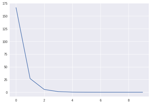
We can also check that the learned weights coincide with the true ones
print(np.linalg.norm(m.weights.tensor - W), (m.bias.tensor - B)[0])
> 1.848553648022619e-05 5.69305886743976e-06
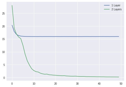
OK, so that was easy, but let's come up with a non-linear dataset, how about $y = x_1 x_2$, we will add a Sigmoid non-linearity and another linear layer to maker our model more expressive. Here we go:
X = np.random.randn(1000, 2)
Y = X[:, 0] * X[:, 1]

losses1 = Learner(
    Sequential(Linear(2, 1)),
    mse_loss,
    SGDOptimizer(lr=0.01)
).fit(X, Y, epochs=50, bs=50)

losses2 = Learner(
    Sequential(
        Linear(2, 10),
        Sigmoid(),
        Linear(10, 1)
    ),
    mse_loss,
    SGDOptimizer(lr=0.3)
).fit(X, Y, epochs=50, bs=50)

plt.plot(losses1)
plt.plot(losses2)
plt.legend(['1 Layer', '2 Layers'])
plt.show()
Wrapping Up
I hope you have found this educative, we only defined three types of layers and one loss function, so there's much more to be done. In a follow-up post, we will implement binary cross entropy loss as well as other non-linear activations to start building more expressive models. Stay tuned...
Reach out on Twitter at @eisenjulian for questions and requests. Thanks for reading!
References
[1] Thinc Deep Learning Library https://github.com/explosion/thinc
[2] PyTorch Tutorial https://pytorch.org/tutorials/beginner/nn_tutorial.html
[3] Calculus on Computational Graphs http://colah.github.io/posts/2015-08-Backprop/
[4] HIPS Autograd https://github.com/HIPS/autograd